|
RDFAnalysis
0.1.1
Physics analysis with ROOT::RDataFrame
|
|
RDFAnalysis
0.1.1
Physics analysis with ROOT::RDataFrame
|
Most users when designing an analysis do not generally care too much about the order in which variables are defined or how to merge the definitions of their various regions into a tree structure. Instead, what you usually wish to have is a set of different regions (defined by selections on the dataset) and histograms (or similar) filled from within each of those regions. The Scheduler is built around these assumptions.
Rather than explicitly building the tree structure through Define and Filter calls, and adding histograms through Fill calls, with the scheduler you instead tell it about all variables, filters and fills you want to use using the registerVariable, registerFilter and registerFill functions. Then, you define new regions using the addRegion function and add fills to those regions using the addFill function. Finally, you schedule the full computational graph using the schedule function.
The output writer can write from a Scheduler directly. When doing this, rather than the nested tree structure used before each region will be written to a separated directory.
The scheduling works in three phases. First a 'raw' schedule is constructed that merges together all the region definitions into a single tree. Then, the Scheduler calculates the necessary order in which to insert any dependencies before each point in the raw schedule. Finally, the scheduler performs the corresponding Define, Filter and Fill calls following the calculated graph.
Note that due to the lazy nature of RDataFrame Define calls, all variables are scheduled at the very start of the graph. Anything that depends on a variable then acquires all of that variable's dependencies. This ensures no variable is evaluated on an event where it is not valid.
When building the computational graph the Scheduler considers all defined variables, filters and fills together. We call these things 'Actions' (not to be confused with what ROOT::RDF::RNode terms Actions), represented by the RDFAnalysis::SchedulerBase::Action class.
Each action has a list of dependencies - these are the variables used as inputs to the operation and any selections necessary to make them valid. For instance the calculation "m_ee = (Electrons.at(0)+Electrons.at(1)).M()" depends on the 'Electrons' variable and some selection that ensures that there are at least two electrons. Each action has both direct dependencies like these but also indirect dependencies (each dependency's own direct dependencies). The variable dependencies can usually be deduced from the structure of the call and filter dependencies are specified as extra argument at the end of the call.
When building the computational graph the scheduler will add all dependencies of a particular action in before it. This allows easy creation of a histogram with preselections, just by listing the preselection as a filter dependency.
Costs allow slightly more control over the order in which actions are scheduled. Lower cost actions will be scheduled earlier than higher cost actions. This can be used to fine-tune the output schedule. Normally this will not be too necessary.
One subtlety involved in job scheduling is that filters are often not independent - one filter can satisfy another. For example, the selection x == 4 clearly satisfies the selection x > 2. At best, scheduling x > 2 after x == 4 wastes CPU time. At worst (when weights are involved) it can result in the double-counting of scale factors.
You can indicate to the scheduler that one filter satisfies another using the filterSatisfies function. Note that these satisfaction relations are transitive: if A satisfies B and B satisfies C then the scheduler will work out that A also satisfies C. More detail is provided in the advanced example.
Returning to the same example used before, this would be set up using the scheduler as
This will produce exactly the same graph as in the previous example.
In order to demonstrate some of the more advanced concepts than those that have already been seen we now consider attempting to reconstruct a H→bb decay. We want to plot the kinematics of both b-jets (where they exist) as well as the mass of the bb pair - for all events as well as those with exactly two b-tagged jets.
Assuming an input dataset
In order to make calculating the scale factors easier we define a few extra functions
Note that ROOT converts std::vectors to ROOT::VecOps::RVecs internally.
Then inside the main function, define the variables and schedule the regions as before
This produces the following computational graph.
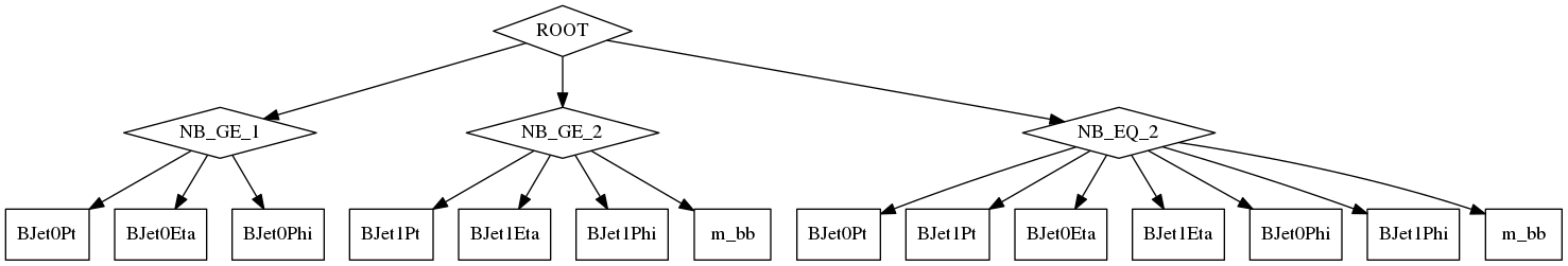
When using filters that involving scale factors (and therefore increase event-level weights) you need to be careful. If, in the advanced example, we had not provided the filterSatisfies relations then to produce the signal region m_bb distribution all 3 filters ("NB_GE_1", "NB_GE_2" and "NB_EQ_2") would have been applied and scale factors up to and including the first b-jet would have been triple-counted and scale factors from there to the second b-jet double counted! However, properly specifying these satisfaction relations fixes this problem.
Another thing to watch out for is the order in which actions are registered with the scheduler. With one exception actions can be declared in any order, that exception being where new (i.e. not present in the input dataset) variables are used in string expressions. A specialised IBranchNamer class is used to extract variables from string expressions, but this only knows about variables after they have been registered. This means that it's always better to register variables first, and to be careful with the ordering of those variables.
 1.8.11
