Introduction

The Node class acts as a wrapper around the ROOT::RDF::RNode class. It provides a similar interface for Filter, Define and Fill. Most of the other actions are not currently implemented but they can easily be added in.

In order to create the root node of your computational tree you should use the createROOT function. All other new nodes will be created by calls to Filter.

Differences to ROOT's RNode

From this brief introduction it may sound like there's no reason to use the RDFAnalysis::Node class over the ROOT::RDF::RNode class it wraps. However the new class adds several new concepts omitted from the other. Many of these will be elaborated on in the Node Concepts section

Weights: ROOT::RDF::RNode has no internal concepts of weights being attached to analysis nodes. Weights can be added manually to histogram fill calls, but the default implementation of cutflows cannot be weighted.

Additionally, it is not easy to deal with event-level weights that change throughout the computational tree, for example due to selections on variables that have associated scale factors.
Navigation through the computational tree: In the older class it is not possible to navigate from a node to its parent or children in the tree. In the new class this is done using the parent and children functions.
Storing filled histograms (and other TObjects) natively in the data structure: With the older class the outputs of actions must be stored somewhere external by the user. Here, the results of fill calls are saved onto the Nodes themselves. Similarly, the Detail template allows for storing arbitrary information in the tree data structure.
Systematics: The older class has no native understanding of systematics, whereas this class is built directly around them. The implementation of systematics is necessarily more complicated so it has its own dedicated page.
Only Filters create new nodes: For the old class all new transformations (defines and filters) created new nodes which can lead to some confusing outcomes. What actually matters for the tree model of the analysis is that the computational graph splits where multiple different filters must be applied to the same input. There is no gain in allowing a new define call to split the graph.
Define multiple variables in a single call: In the old class it isn't possible to define multiple variables in one call - each variable requires a separate call. This is enabled in this class through the Define overload accepting a std::array.

Node Concepts

Branch Namers

Each node has a branch namer object which keeps track of the branches defined at that point in the analysis. This is mainly used for systematic variations (so will be covered on the dedicated page) but is also used to work out which variables are used in string expressions.

Weights

Each Node has its own weight, accessed through the getWeight function. These weights are applied to the weighted cutflow, as well as to any histogram fill calls. Extra arguments can be added to all Filter and Fill calls to set up changing the weights used in those calls. As with Define and Filter calls, these weights can be calculated either with a C++ function-like object or using a JIT compiled string expression.

Additionally a WeightStrategy can be specified. This tells the Node how it should apply this weight. There are two main options to be configured: whether or not the weight added by this node should be multiplied by the weight of the node before it and whether or not this should weight should be applied always or only in 'MC' mode. MC mode is a setting for the whole computational graph, set in the createROOT function, which allows turning off all weights that have the MCOnly WeightStrategy, for example, in order to run on data which does not have those weights. The default value for the WeightStrategy is to be both multiplicative and MC-only.

Detail

The Node class has a 'Detail' template parameter. This is used to add extra information (i.e. not histograms) to be stored within the data structure. This defaults to the EmptyDetail class which adds no extra information.

An example of extra information that you might want to add is provided by the CutflowDetail class, which stores information about the number of events passing each filter.

Each node's detail is accessed via the detail function.

Run Monitors

You can manually trigger the event loop using the run function. This function can take a template parameter called a Monitor. This object must define an operator() taking a single unsigned int parameter, which is the slot number. This will be provided to the ForEachSlot function of the root of the computation graph (only the nominal variation, if systematic variations are present). Alternatively, a print interval and (optional) total number of events can be provided and the default RDFAnalysis::RunMonitor will be used.

If you do not want to use this feature, then you can trigger the loop implicitly by trying write out from the result of any of the fill actions.

Output Writers

In order to write out the information stored in the tree structure you could manually recurse through the tree and write out how you choose. However, the package also provides the OutputWriter class to write out objects for you.

The OutputWriter mirrors the tree structure of the analysis in the output ROOT file with nested directories representing each step in the computation. The output to be written from each node is decided by adding INodeWriters to the OutputWriter. These decide what information to write from each node and how.

Two of these are pre-written. The TObjectWriter writes the output of all Fill actions. The CutflowWriter converts the information stored in the CutflowDetail into a cutflow, therefore in order to use this class the Detail type of the node must at least inherit from CutflowDetail.

Usage Example

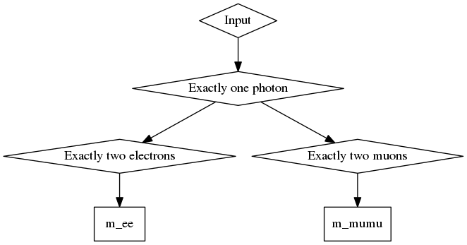
Returning to Zγ example used earlier, assuming that the input TTree contains three branches

std::vector<TLorentzVector> Photons;
std::vector<TLorentzVector> Electrons;
std::vector<TLorentzVector> Muons;

containing the kinematics of all photons, electrons and muons passing certain object-level selections, then the corresponding code snippet to create the computational graph and write out the histograms would be (assuming an input ROOT::RDataFrame object called inputDF):

using node_t = RDFAnalysis::Node<CutflowDetail>;
std::unique_ptr<node_t> root = node_t::createROOT(
    inputDF, //> The input to this analysis
    std::make_unique<RDFAnalysis::DefaultBranchNamer>({"NOSYS"}), //> Systematics related
    false //> run without weights
    );
node_t* photonSelection = root->Filter("Photons.size() == 1", "N_GAM_1", "Exactly one photon");
photonSelection->
  Filter("Electrons.size() == 2", "N_ELE_2", "Exactly two electrons")->
  Define("m_ee", "(Electrons.at(0) + Electrons.at(1)).M() )")->
  Fill(TH1F("m_ee", ";m_{ee} [GeV]", 50, 50, 100), {"m_ee"});
photonSelection->
  Filter("Muons.size() == 2", "N_MU_2", "Exactly two muons")->
  Define("m_mumu", "(Muons.at(0) + Muons.at(1)).M() )")->
  Fill(TH1F("m_mumu", ";m_{#mu#mu} [GeV]", 50, 50, 100), {"m_mumu"});
RDFAnalysis::OutputWriter<node_t::detail_t> writer("output.root");
writer.addWriter<RDFAnalysis::CutflowWriter>();
writer.addWriter<RDFAnalysis::TObjectWriter>();
writer.write(*root);

This will produce a computation graph that looks like